VOLUME 6: Table of Contents
TEACHING ISSUES AND EXPERIMENTS IN ECOLOGY
TEACHING
ALL VOLUMES
SUBMIT WORK
SEARCH

Comments by Contributing Authors — Christopher A. Lepczyk
Challenges to Anticipate and Solve
- Interest among all students. Not all students enjoyed this topic of study. The solution to this challenge was to discuss in general terms why it was important to study, to try and have students ask additional subquestions to the main question, and to ask for student input on what they would have preferred to investigate.
- Semester long project. Most students enjoyed having one large theme to work on all semester, but a handful of students indicated that they would have liked individual labs each week. One of the few solutions to this was to have several separate labs that were not part of the synthetic question. Ultimately, this was the single biggest challenge because students did not like having so much of their time and grade devoted to an overarching synthetic perspective.
- Poster presentations. Students very much enjoyed creating a poster for their project, but several had little experience with graphical design or software used for poster layouts (e.g., MS PowerPoint). Because students worked in groups, however, peer-to-peer learning generally resolved this issue. Notably, providing a short lecture or demonstration on how to layout posters in PowerPoint at the same as going over general guidelines would be beneficial. One other issue that can arise with posters is the length of time needed to print them out. Students may need several days or a week to have them printed, depending upon location and resources. A simple alternative that I used was to have students project their posters onto a screen just like it was a real printed poster. This solution eliminates printing and the associated time and money associated with it.
- Data analysis. Most students were able to conduct the statistical analysis either by themselves or at least in their groups. However, some individuals did not understand the output from SPSS. Both the teaching assistants and I worked to resolve this lack of understanding by going over the results with any student that had trouble understanding them. It is important to anticipate that a given percentage of students will have some difficulty in understanding statistics and what the results mean (both numerically and ecologically). Thus, the instructor should be prepared to go over the statistics used and results in some detail with individual students that are struggling.
- Differences in student knowledge and ability. Although the lab was designed for a 300 level course, students coming into Ecology had a very wide range of backgrounds. For some, the lab was almost too simple (about 10% of students), whereas for about 20% of the students, it was essentially overwhelming. As with any course, trying to find the level and bar to set for students to think and achieve is the main challenge. The solution was to have a number of items turned in to the instructor/TA as a draft and evaluated so that the student could improve the specific item before they were actually graded. In addition, instructors and TAs offered extra lab time and office hours to work with students.
<top>
Introducing the Experiment to Your Students
I introduced the semester project in the second lab by discussing general ecological principles and how we collect data to continue to support or refute them. Then I moved into a discussion of how one current pattern (i.e. the rural-urban gradient) has been shown to have three different relationships (Figure 1). I briefly discuss these three relationships, what they mean, and what some possible explanations may be for the given relationship. While I provided this information on the three relationships when I taught the laboratory, it can easily be modified to make the course more inquiry based. For instance, students could be required to draw out the three general relationships that are described by the hypotheses and illustrated in Figure 1. Following this exercise, students could then conduct a literature review and answer a set of questions (a sample of which are illustrated in the Questions for Further Thought above) that require them to understand the mechanisms responsible for the three different relationships. In addition, students could be asked to find other human influence measures in the literature (e.g., anthropogenic noise, pedestrian traffic) or come up with them in class and discuss how they might relate to species diversity. Depending upon the type of class, different measures of diversity could also be considered. A second component of introducing the lab is to discuss how ecologists assess (i.e. measure) human influence. In the class I taught I explained the general measures of human influence and gave some examples of what either end of the continuum might look like. However, because the human influence gradient is relative, it is important to note how human influence can be measured at each point along the gradient. For instance, the instructor could go over how to count number of cars or people that pass by a site in a given amount of time (similar to Blair 1996). By conducting specific measures of human influence at each site, students can also compare their data with other published results or other classes, if time allows or if multiple years of the experiment are conducted.
<top>
Experiment Description
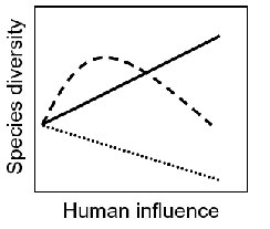
Figure 1. Competing hypotheses relating species diversity and human influence (i.e., population, houses, land cover, etc.): Productivity (solid line), Intermediate Disturbance (dashed line), and Ecosystem Stress (dotted line) from Lepczyk et al. 2008.
Introducing the Experiment to Your Students:
Each week during the field sampling portion of the laboratory, the groups of students would collect information on trees and birds. Depending upon the field site and amount of time needed to collect the data a given group might collect only data on trees or birds for a given lab period, or they might collect information on both. For trees, groups laid out a 10 m by 10 m plot using a compass and measuring tape. The plot should be as close to square as possible. Groups then identified all tree species in the plot to species level (if possible) using the taxonomic keys and field guides provided (if unable to identify in the field, students were able to bring plant material back to campus for further inspection). For each species students recorded the common and scientific names as well as the diameter at breast height (dbh). To measure dbh students found the point on the tree trunk where their sternum would touch if they stood next to it. Then using a tape measure, the students determine the diameter to the nearest mm (if possible). Dbh is measured in order to be able to determine each tree’s biomass through an allometric equation.
For bird censuses, point counts were used following the standards established by BBIRD. Under this protocol surveys are carried out for 10 minutes within a 50 m fixed-radius circle. We used a 50 m circle in order to allow comparability among widely different habitat types and to maximize the probability that bird counts reflect vegetation measured at the point. However, all birds detected beyond 50 m should also be recorded to allow total detection of species. All birds were recorded and distinguished by male, female, or unknown for each individual bird detected and distinguish between birds inside and outside of the 50 m radius circle. Once a survey was completed, a group moved to a new location that was a minimum of 200 meters away. The instructor and teaching assistants assisted with bird identifications and counts. One important consideration of the bird counts to note to students and instructors is that the time of day that birds are counted can greatly influence the bird species present. Hence, an afternoon count could yield very different compositions of species than an early morning count. To reduce any confounding factors the bird censuses should be conducted at the same time of the day throughout the semester.
After the bird and tree data were collected, the students entered the information into MS Excel spreadsheets in the computer lab (if possible during the end of the laboratory period). All groups followed the same data entry procedure, which included columns for the group name, the field site location, the plot or point count number, common name, species name, and abundance. At the same time students also created a separate spreadsheet page that listed all of the metadata (e.g., descriptions of the field sites, any abbreviations used). After the field data were entered, students added new columns to their group’s spreadsheet that identified if a species was native or exotic, the mass or biomass for a species, the total mass or biomass of a plot, the native mass or biomass of a plot, the exotic mass or biomass of a plot, the relative abundance of a species in the plot, the richness of all species in a plot, the richness of the native species in a plot, the richness of exotic species in a plot, the Shannon diversity of a plot, and the Shannon evenness of the plot. Bird masses were provided by the instructor from Dunning 1992. Students calculated the biomass for each tree by using allometric equations from Jenkins et al. 2003 that use the dbh estimate and generic tree classifications to estimate a tree’s biomass. When all field sites had been entered by all groups, the instructor edited and compiled a master database for trees and a master database for birds from all 16 groups. These databases were placed on the course website so all students could access and use them as needed.
Prior to conducting statistical analyses, the entire class discussed the completed data and where they had been collected. This allowed the students to define the gradient as a relative scheme of plots from fairly pristine to most developed that all students could agree upon (and to which the instructor concurred). In defining the gradient, the students used amount of impervious surface, land use (e.g., residential, commercial, park, etc.), and qualitative views of such factors as anthropogenic noise, traffic, and presence of people. Once the gradient was finalized, students coded the gradient from 1 to 6, with the former being the most pristine, thereby allowing for regression analysis. In order to help guide students on the regression exercise I used a graphic similar to Figure 1 and discussed which type of model would describe each of the three lines with each lab section during the day of analysis. Specifically, we discussed how a linear model could support either the Productivity or Ecosystem Stress Hypothesis as well as how a quadratic model could support any of the three hypotheses, depending upon the location of the parabola’s apex. Then, within groups, the students converted the Excel data into SPSS data and conducted linear and quadratic regressions of the data. For instance, students investigated how total species richness, native species richness, and exotic species richness changed over the gradient. After the regressions were run, students compared whether a linear or quadratic model was better by comparing adjusted r2 values, p-values and figures of the linear and quadratic models. In summarizing all of the results, students compared the linear and quadratic models, as well as if any model was significant.
The basic design of the analysis is set-up to allow students to compare whether a relationship exists between the diversity measures and the human influence measures. If a relationship does exist according to the statistical results, the students need to understand (often through graphing the result in conjunction with the formal statistics) and interpret which hypothesis is supported. Because the three hypotheses are essentially an increasing, decreasing, or negative parabolic relationship, it is fairly straightforward for students to interpret the results to each hypothesis. If a number of different taxa or diversity measures are being investigated, then it is important to have students consider which hypothesis has the most or predominate amount of support.
Data collection for this lab can vary greatly, depending upon what taxa the instructor or students are interested in studying. The most important portions were to describe how to lay out plots, conduct biological inventories, enter data into Excel, and work with computer software. In addition, it would be beneficial to discuss aspects of quality assurance and quality control (QA/QC) and metadata early on in the semester (if not even before field work begins) in order to give students a broader appreciation of the value and importance of their data.
- Depending upon the course and institution, the laboratory Methods and Materials can be altered to be more inquiry based than presented. For instance, rather than layout all of the study sites and specific types of data collected, students could be asked to determine what type of data they are going to collect, how they would conduct the specific measurements, how many sites they should collect from, and why these are important aspects. Such inquiry could lead to discussions of experimental design, sample size, replication, sampling methodology, and field methods.
Formulas Used in the Laboratory
Species Richness: the sum of all unique species in a given plot.
Relative Abundance: the proportion (pi) of a species abundance relative to the total abundance of all species.
Shannon Diversity (H'): H' = -∑piln(pi), where H' = the Shannon Diversity index, pi = the proportion of the ith species, and ln = natural log. The summation is for all species in a given grouping.
Shannon Evenness (J'): J' = H'/ln(S), where S = the number of unique species (i.e., richness)
Tree biomass: bm = Exp(β0 + β1lndbh); where bm = total aboveground biomass (kg dry weight) for trees 2.5 cm dbh and larger, dbh = diameter at breast height (cm), Exp = exponential function, and ln = natural log. Estimates for β0 and β1 can be found by tree groupings in Jenkins et al. 2003.
<top>
Questions for Further Thought
- How do humans influence native species?
Depending upon what students find, it could certainly be positive, intermediate, or negative. In the case of my course, the birds generally supported the ecosystem stress hypothesis as native species declined and exotic species increased. However, trees did show more variance.
- Which species benefit from human influence and which do not?
Depends upon the location, but it is interesting for students to consider which factors may lead to a species benefiting from influence. This can lead to many other questions about synanthropy, species endangerment, etc.
- What does the preponderance of evidence suggest about how humans influence individual species, populations, and communities?
Likely to indicate that humans are detrimental, but again will depend upon how gradient is laid out, species sampled, etc.
- Is a rural-to-urban gradient the same as a pristine-to-human dominated gradient?
This question depends upon the depth to which students have reviewed the topic in the literature as well as how much they may have thought about the project. Within my class several students were able to note that we can measure human influences in many different ways and they suggested this might influence the outcome of the gradient. However, students could have gained a broader understanding of this question if it was posed as an open discussion topic at the end of the semester.
- Does the total plant or animal biomass change in relation to the location on the gradient?
To answer this question the students needed to look through the results of their regression models. During the analysis portion of the lab, students calculated linear and quadratic regressions of total biomass, native biomass, and exotic biomass from trees and birds separately. All groups found that total bird biomass decreased significantly over the gradient, but that total tree biomass showed no significant trend (it did however decrease non-significantly). One misconception with understanding these changes along the gradient were if they were significant or not (i.e. the pattern suggested a relationship, but the statistical result indicated no significant relationship). Other misconceptions included remembering the differences between native and exotic species.
- Based upon our findings, is there any guidance we an offer about the continued development of land around the world or urban sprawl?
A major finding of the study was that native species and total species richness, diversity, evenness, and biomass decreased with increasing levels of human influence for one or both taxonomic groups. Tree and birds did differ from one another, but the preponderance of evidence suggested that human land development was not beneficial to most species or biodiversity. Generally, the result found by students did not lead to any misconceptions. If anything it solidified what a number had suspected about the negative ramifications of urbanization or land development.
<top>
Assessment of Student Learning Outcomes
I used three major pieces of assessment for this lab, which ultimately I believe may have been too few. Breaking out a few more aspects for separate grades or more in-depth consideration would likely have been beneficial for students. Similarly, spreading out the assessments over a wider portion of the semester, instead of coming predominately at the end, would have been beneficial for students. Comments on each assessment aspect are listed below:
Field Notebook. The field notebook was a very positive experience for all students. Many liked using Rite in the Rain books (especially when it did rain!) and learning to record field information. By grading the notebooks after two field labs, students were able to vastly improve their skills and continued to hone their note taking skills. Furthermore, the teaching assistants and I were able to look at individual improvement over several field trips. In retrospect I would have graded the notebooks three times instead of twice. In addition, while students did receive a lecture and handout on biological monitoring and field data collection, I would provide either photocopies or additional handouts on what an “ideal” field notebook should look like.
Poster. Students found the poster presentation to be the best of the three assessment tools. They enjoyed learning how to use MS PowerPoint or MS FrontPage to create a visual document and how their vision compared to other groups. Main issues that I dealt with were showing students how to tell a story visually while also including the relevant content and figures. Students also appreciated that their independent grades were an amalgam of their peers and the instructors, thus slightly limiting the ability of any one person from sinking their overall grade. Although I did not evaluate a draft version of each group’s poster, this could also be done to allow for both improvement and wider grade dispersion.
Paper. The synthetic paper in the style of Ecology was the main component of the course and ultimately was both a very positive tool and also a very difficult one. Successful students put a great deal of time into their work and produced papers that were written in a scientific style, included a number of additional citations, and looked like draft papers from an MS thesis. On the other hand, for students that were weak writers, the paper was very challenging and a source of great frustration. Having students do drafts of other sections and perhaps even critiquing each others (an opportunity to talk about peer review as well) would have been useful. Similarly, offering students the opportunity to revise a section like the Methodology or Introduction several times would have been beneficial to a handful of students. Finally, I used a system of grading the draft sections of the Introduction and Methods that was simply a check minus, check, or check plus to indicate the level that a student had achieved. Upon reflection I would have the draft sections of the paper count either as a completely separate grade or as a percent of the final paper grade.
<top>
Evaluation of the Lab Activity
Because this particular laboratory requires most, if not all semester, the students have a variety of thoughts on its value. After running this laboratory for the first time I handed out an evaluation form (a copy of this evaluation can be found under the download section and is entitled “Student Evaluation of Lab Semester Research Project”). In general, the overall majority (61%) of students liked the approach of one long project and enjoyed being in the field doing real science. Similarly, ~71% of the students would recommend this laboratory to others in the future. While there were legitimate criticisms of certain aspects of the lab (e.g., amount of time to get to a field site), most of what students disliked about the lab are common among any lab exercise or class. For instance, many students disliked analyzing the data, having to collect multiple samples, and working in groups.
Based upon this evaluation, students had the following thoughts to the questions:
-
Did you like doing one large semester project?
YES = 61.1% (44/72) vs. NO = 25%
(18/72), with the remainder being undecided or not answering. Interestingly, half of the NO students (n = 9) were all from the first lab session, which began at 8:00 AM and was the last choice lab section every year according to previous instructors. Hence, it is likely a portion of this group would have been dissatisfied with any lab option. - What did you like best about the lab?
The most common answer was working outside/field trips, followed by such reasons as: that it was a real world lab/real scientific project, collecting field data (hands-on), the uniqueness of the semester long approach, working in groups, working on an interesting topic, topics were well explained, the interactive nature of lab sessions, and not having quizzes. - What did you like least about the lab?
Common answers included: data entry and analysis, having a lot of work due at the end of the semester, group project, not understanding the labs or the overall goal of the project, having to conduct the same type of inventories at multiple locations (repetitive), boring and filled with busywork, not having enough time, the research paper, too many field trips (being outside), too many separate tasks, the lack of many lectures in lab, using new software (i.e. MS Excel, SPSS) and computers, too much work for a 300 level class. - Question 4 contained 15 subquestions, with response options ranging from Greatly Disliked (1) to Greatly Liked (5). The following are mean responses based on 72 responses as follows:
4a. First week field trip around Milwaukee: 3.86
4b. Weekday field trips (UEC, Campus, etc.): 4.32
4c. Weekend field trip to UWM Field Station: 3.85
4d. Learning to count birds: 3.64
4e. Learning to count trees: 3.71
4h. Learning to use Excel: 3.60
4i. Learning to enter metadata: 3.24
4j. Learning to conduct scientific literature review: 3.15
4k. Learning to use a statistics program: 3.24
4l. Learning new types of software: 3.50
4m. Learning to make a poster presentation: 3.49
4n. Learning to use a field notebook: 3.78
4o. Learning to write a scientific paper: 3.34
- Would you recommend this laboratory to other students?
YES = 70.8% (51/72) NO = 20.8% (15/72) NO OPINION = 8.3% (6/72)
Overall, most students found each major aspect of the course to be a positive experience. However, considering these comments, there are aspects of the laboratory that would benefit from modification in the future. First, splitting the graded components up over the semester would help some students from feeling so overwhelmed at the end. Second, spend a bit more time on explaining the need for replication and the value in having many people collect data. Third, I would integrate the literature review component into the lab and have them use the literature to more depth.
<top>
Translating the Activity to Other Institutional Scales or Locations
(1) The lab is easily conducted at large or small institutions and can be expanded or reduced by an instructor to meet their course needs very easily. Essentially, many aspects of the lab can be parceled out into smaller components that answer separate questions and have graded components or more aspects can be added. For instance, the gradient paradigm presented here can be simplified by an instructor or even used with preexisting data collected from all or part of the gradient if time does not allow for a full semester project. In particular, the data provided with this laboratory can be used over the course of one or two lab sections to answer several questions if an instructor is so interested.
(2) The lab can easily be conducted in any location around the world where there is a human influence gradient. Similarly, the lab can be run using many different taxa, although they should be terrestrial species. Finally, the lab can be run at different times of the year as long as the instructor is aware of the types of species present in a given season. However, winter is probably the least opportune time to conduct the lab for both students and the species that can be censused.
(3) The only limitation for physical disability is dependent upon the field location. In regards to learning disabilities, this exercise may be more challenging for students that have short attention spans as it is a long term project with benchmarks.
(4) This lab can be simplified and/or shortened to teach to pre college levels by removing some of the multiple sampling within sites and/or focusing on only a single taxonomic group. If used in a pre college level, the laboratory may require that the instructor spend additional time to review the background literature in order to fully understand the scope of the questions. Essentially the instructor would need to assess the specific class that he or she wishes to use this laboratory for and adjust it accordingly.
(5) Several aspects of the laboratory ultimately depend upon a specific institution’s guidelines for laboratory exercises. For instance, institutions vary on whether or not they allow students to drive themselves to a field site for a class requirement.
(6) Conducting a laboratory of this scale certainly benefits from having a teaching assistant. However, it should be noted that this ultimately depends upon how many students are present in a laboratory section, how much travel would be necessary, and how in-depth the instructor would like to make the laboratory.
<top>