AUTHORS
Anna L. Carter
Department of Ecology, Evolution & Organismal Biology, Iowa State University (acarter1@iastate.edu)
THE ECOLOGICAL QUESTION
How are abiotic environmental conditions associated with a species’ geographic distribution?
ECOLOGICAL CONTENT
species distributions, habitat suitability
WHAT STUDENTS DO
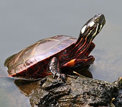
Students use R to search, download, and plot the distribution of painted turtles from the Global Biodiversity Information Facility (GBIF), then implement the BioClim modeling algorithm to build an occurrence-based species distribution model for painted turtles using the BioClim variables.
SKILLS
Geospatial/mapping skills, R/command-line skills, data manipulation and plotting of large spatial datasets, introductory distribution modeling, searching public databases
STUDENT-ACTIVE APPROACHES
Cooperative learning: Students can work through the exercises in groups, using either the painted turtle data or group-specific taxa (i.e., each group selects a taxon to model). This module addresses multiple, complex concepts – online data availability & access, spatial query & analysis, global climate models, theoretical concepts of SDMs, model fitting – any of which can be expanded depending on the instructor’s preference, group work can be especially beneficial for facilitating comprehension and may be more efficient.
Jigsaw: The module can be easily extended to allow each student/group to examine the distribution of a different species and explore data availability among taxa as well as different aspects of model fitting.
ASSESSABLE OUTCOMES
In addition to using the provided student handout as an assessment tool, instructors can use the provided short-answer questions to build essay assessments, highlighting aspects of the material that are of particular interest to the course as a whole. Through completion of the module material students should be able to:
- Identify publically-accessible sources of occurrence records for different species and discuss the attribute data that are associated with those records.
- Visualize and describe spatial patterns in occurrence data.
- Identify the types and structure of data available in climate/bioclimate layers and discuss how those data are selected for building SDMs.
- Explain how the Bioclim algorithm fits species occurrence records.
- Discuss differences between presence-only and presence-absence SDMs and some of the strengths/limitations of each.
SOURCES
- GBIF database [https://www.gbif.org/]
- WorldClim database [https://www.worldclim.org/bioclim]
- US Census Bureau [https://www.census.gov/geo/maps-data/data/cbf/cbf_state.html]
DOWNLOADS
- Full Article Text [docx], [pdf]
- a folder containing a .shp file and associated metadata for plotting a 20m map of US states, downloaded from the US Census Bureau [https://www.census.gov/geo/maps-data/data/cbf/cbf_state.html]. This is the only file that students need to be provided. The remaining files are for instructor reference only.: usa.zip
- cleaned version of the painted turtle occurrence records that students download from the GBIF database [https://www.gbif/org]: occur.csv.
- a folder containing .png files of the five maps students create during the exercise: maps.zip
- R code for completing the exercises, copied from the student handout: painting_turtles.R
Description of Excel Files:
All the data used in this module are freely available online.
ACKNOWLEDGMENTS
The author is supported by National Science Foundation grants DEB-1242510 and IOS-1257857 and the Minnesota Herpetological Society. This exercise draws heavily from the vignettes found in “Species distribution modeling with R” by Hijmans & Elith (2017).
CITATION
Anna L. Carter. November 2017, posting date. Painting turtles: an introduction to species distribution modeling in R. Teaching Issues and Experiments in Ecology, Vol. 13: Practice #1 [online]. https://tiee.esa.org/vol/v13/issues/data_sets/carter/abstract.html
